Publications / Latency-Aware Routing

Beyond Accuracy and Cost: Latency-Aware LLM Query Routing for Dynamic Workloads

Shivam Patel^1†, Akaash R. Parthasarathy^1†, Ankur Mallick², Gauri Joshi¹

¹Carnegie Mellon University   ²Microsoft† Equal contribution

arXivarXivPDFCode

Bridging two sides of the routing decision

A language query router assigns each prompt to a model. Existing routing methods typically focus on two quantities. Accuracy estimates the quality of the resulting response from historical query–model evaluations, while cost is largely determined by token counts and published prices. By sending easier queries to smaller, less expensive models and harder queries to larger models, a heterogeneous model pool can achieve a better quality–cost tradeoff than any single model in the pool.

What these methods generally do not model is when the response arrives. Most query routers are latency-agnostic: they select the instance with the best predicted accuracy–cost utility without accounting for its current workload. When similar queries repeatedly prefer the same model instance, traffic can concentrate on that instance and produce substantial queueing delays.

The systems literature addresses the complementary problem. Load-balancing policies across replicas — such as round-robin and join-the-shortest-queue — and schedulers that prioritise requests by deadline or predicted output length can effectively control latency, but they operate under a fixed query-to-model assignment. They decide which replica should serve a request, rather than which model should answer it, and are therefore accuracy- and cost-agnostic by construction.

These two decisions are usually made independently. This work bridges them through a single routing decision that jointly optimises accuracy, cost, and latency.

Why decoupled routing fails

The interactive example below considers a small deployment with one instance of each of three Qwen3 models, a query stream drawn from four tasks with distinct prompt and response length distributions, and the same arrival trace evaluated under four routing policies. The accuracy scores and per-token prices match those used in the paper, so the routers optimise the same accuracy–cost utility considered in our experiments.

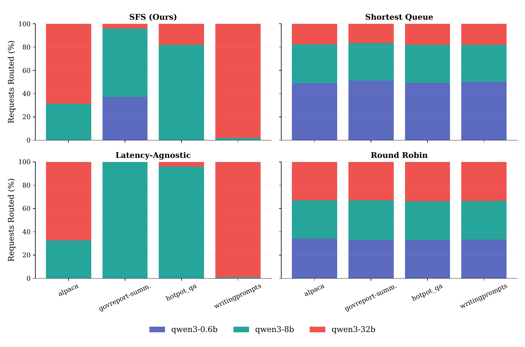
The three instances are assigned identical service capacity. This is intentionally not representative of the physical throughput differences between 0.6B and 32B models; instead, it isolates the effect of the routing policy by ensuring that differences in latency arise from query assignment rather than heterogeneous service rates. Under these prices and quality scores, Qwen3-0.6B is never the utility-maximising model for any of the four tasks.

Interactive · one arrival trace, three model instances, four routers

Router

Arrival rate 6 q/s

one query — solid = tokens computed, dashed = still to come, tick = prompt ends the solid part is coloured by where the query stands against its TTFT target: still waiting for its first token first token arrived on time first token arrived too late

Every router on the same arrival trace

Router	Mean TTFT	p95 TTFT	On time	Utility	OnTimeUtility

Time-to-first-token, selected router

All three instances are assigned identical service capacity in this demonstration, so any latency differences arise solely from the routing policy rather than from differences in model serving speed; each model is deployed on a single instance. Prompt and response lengths are chosen to represent the four task regimes — short/long prompts crossed with short/long responses — rather than sampled directly from the measured distributions, and are scaled so that the paper's TTFT targets remain feasible on an idle instance. Accuracy values are taken from the paper's LLM-as-a-judge evaluations, while costs use published Qwen3 per-token prices, so the accuracy–cost utility optimized by each router is unchanged. Under these utilities, Qwen3-0.6B is never the utility-maximising choice for any of the four tasks; consequently, an accuracy–cost-only router leaves it idle even as the preferred instances become saturated. The engine shown here is a token-batch simulator, and SFS evaluates each routing decision by rolling that simulator forward from the current workload of each instance using predicted decode lengths (with ±30% error). The simulation is therefore intentionally close to the estimator's internal model; the paper separately validates this approximation against a real vLLM deployment, where SFS achieves approximately 5% TTFT prediction error.

The accuracy–cost router achieves high unconstrained utility but poor latency. It leaves the 0.6B instance unused and concentrates long-prompt summarisation traffic on the 8B instance, whose queue grows steadily; by the end of the trace, tail latency is measured in seconds despite targets of only hundreds of milliseconds. In contrast, Shortest Queue maintains low latency by distributing requests across instances, but because it is unaware of query–model utility, realised utility decreases substantially. SFS is the only policy in the example that simultaneously maintains high utility and low latency. This tradeoff is captured by OnTimeUtility: the realised accuracy–cost utility, with queries that violate their latency targets assigned zero utility.

At sufficiently high arrival rates, all policies eventually saturate. This highlights an important limitation: routing reallocates available capacity but cannot create additional capacity. Above roughly 9 q/s in this illustrative three-instance deployment, the offered load exceeds what the pool can sustain, and additional serving capacity is required.

Decomposing time-to-first-token

We optimise time-to-first-token (TTFT), defined as the interval between a query’s arrival and generation of its first output token. TTFT directly captures responsiveness for interactive applications. For query $q_i$ assigned to model instance $j$, it decomposes into two components:

\[L^{\text{ttft}}_{i,j} \;=\; W_{i,j} \;+\; P_{i,j}\]

where $W_{i,j}$ is the waiting time before the query’s prefill computation begins, during which it waits for compute and KV-cache memory occupied by earlier requests, and $P_{i,j}$ is the time required to process its prompt and generate the first output token.

TTFT under continuous batching. A new sequence $q_i$ arrives at time $t$ (left), its prefill computation begins at $t + W_{i,j}$ (centre), and its first decode token is generated at $t + W_{i,j} + P_{i,j}$ (right). Each column represents one token batch, which may combine at most one decode token per active sequence with prefill chunks from sequences whose prompts are still being processed.

Why the serving framework matters

Autoregressive generation consists of two phases with different hardware characteristics. Prefill processes prompt tokens in parallel to populate the KV cache and is typically compute-bound. Decode generates output tokens sequentially, with each step reading cached keys and values from prior tokens, and is typically memory-bound.

Modern serving frameworks interleave these phases rather than executing them as isolated stages. Under continuous batching — used by systems such as ORCA and vLLM — new prompts can be admitted at token-iteration boundaries instead of waiting for an entire sequence-level batch to finish. vLLM’s PagedAttention dynamically allocates KV-cache blocks instead of reserving each sequence’s maximum context length in advance. Sarathi-Serve’s chunked prefill further partitions long prompts and interleaves prefill chunks with decode work, reducing stalls for sequences already generating tokens.

Consequently, a model instance cannot be described by a single fixed service rate. The processing time of the next token batch depends on its composition: the number of decoding sequences, their accumulated context lengths, the size of any scheduled prefill chunk, and the position of that chunk within its prompt. The latency of a newly arriving query therefore depends on the workload state it encounters and on how the serving framework will construct subsequent token batches.

A throughput-based estimator and its limitations

A natural baseline profiles each instance’s prefill throughput $\theta^{\text{pre}}_j$ in tokens per second, sums the outstanding prefill tokens at the instance, and divides:

\[\widehat L_{i,j}^{\textrm{ttft}}(t)= \underbrace{\frac{\sum_{q\in \mathcal{R}_j(t)} \textrm{tok}^{\textrm{pre}}_{q,j}(t)}{\theta^{\textrm{pre}}_j}}_{\text{waiting time}} \;+\; \underbrace{\frac{\textrm{tok}^{\textrm{pre}}_{q_i,j}(t)}{\theta^{\textrm{pre}}_j} + \bar T^{\textrm{dec}}_j}_{\text{prefill and first token}}\]

Here $\mathcal{R}_j(t)$ denotes the resident set at instance $j$ — all queued and actively served requests — while $\bar T^{\text{dec}}_j$ is the average decode-batch time used to approximate the computation of the first output token.

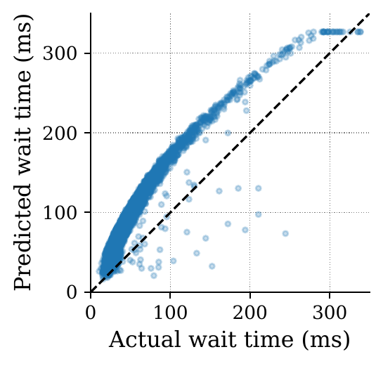
This estimator is simple and intuitive, but it introduces a systematic source of error. A single throughput value is representative only of the batch composition on which it was profiled. A throughput estimate obtained from prefill-dominated batches can substantially underestimate latency when the live instance is simultaneously serving many long-context decode sequences that compete for memory bandwidth. The resulting error is therefore not merely random variation; it is workload-dependent bias that increases as the live batch composition diverges from the profiling workload.

Predicted versus measured TTFT on Qwen3-0.6B hosted on one H100, using the prefill-throughput estimator (left) and the proposed Serving Framework Simulation (right). By ignoring interference from decode work, the throughput estimator yields 85% mean absolute percentage error, whereas SFS models the generation process and reduces the error to 5%. The remaining outliers in both panels are attributable primarily to CPU and kernel overheads.

Serving Framework Simulation

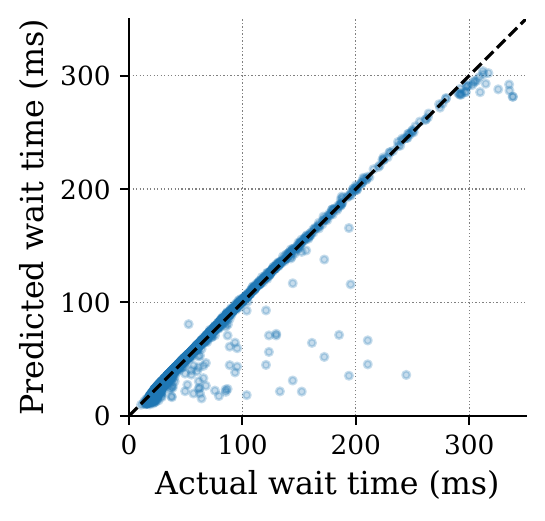
The key observation is that latency can be estimated by explicitly simulating how the serving framework will schedule future token batches. SFS starts from the workload currently resident at an instance, inserts the incoming query, and replays the framework’s batching and scheduling rules until that query produces its first decode token.

Formally, for a query $q_i$ arriving at instance $j$ at time $t$, SFS constructs the augmented workload

\[\mathcal{X}_{i,j}(t) = \left\{\left(\textrm{tok}^{\textrm{pre}}_{q,j}(t), \widehat{\textrm{tok}}^{\textrm{dec}}_{q,j}(t)\right) : q \in \mathcal{R}_j(t)\right\} \cup \left\{\left(\textrm{tok}^{\textrm{pre}}_{q_i,j}(t), \widehat{\textrm{tok}}^{\textrm{dec}}_{q_i,j}(t)\right)\right\}\]

pairing each resident request’s remaining prefill tokens with its predicted remaining decode tokens. From this state, SFS constructs successive token batches according to the serving engine’s policy — at most one decode token per active sequence, together with prefill chunks that fit within the token budget — while respecting queue order, admission limits, context limits, KV-cache allocation, and preemption. Let $\ell^{\text{TTFT}}_j(t,i)$ denote the index of the batch in which $q_i$ emits its first decode token. The TTFT estimate is the sum of predicted batch-processing times up to and including that batch:

\[\widehat{L}^{\textrm{SFS}}_{i,j}(t) \;=\; \sum_{\ell=1}^{\ell^{\textrm{TTFT}}_j(t,i)} \widehat{T}^{(\ell)}_j(t)\]

Two properties keep this simulation lightweight. First, SFS terminates at the incoming query’s first token rather than simulating every resident request to completion, so the simulation horizon is typically short. Second, TTFT estimation is relatively robust to decode-length error because each active sequence contributes at most one decode token to a token batch. The dominant factor is therefore how many sequences remain active during the relevant horizon, rather than their exact eventual output lengths. Errors in predicted response length primarily affect when a sequence departs, which often occurs beyond the short horizon relevant to TTFT.

Estimating the processing time of a token batch

The remaining component is $\widehat{T}^{(\ell)}_j(t)$, the predicted processing time of one token batch. Rather than modelling individual kernels and memory transfers, which can be fragile across workloads, we parameterise batch time using features of the batch composition. For each sequence $q$ in batch $\ell$, let $c_{q,j}(t,\ell)$ denote its context length before the batch executes:

\[\begin{aligned} \widehat T^{(\ell)}_j(t) \;=\;& \beta_{0,j} \;+\; \beta_{1,j}\!\!\sum_{q\in \mathcal{B}^{(\ell)}_j(t)}\!\!\left(\textrm{tok}^{\textrm{pre}}_{q,j} + \textrm{tok}^{\textrm{dec}}_{q,j}\right) \;+\; \beta_{2,j}\!\!\sum_{q\in \mathcal{B}^{(\ell)}_j(t)}\!\! c_{q,j}\,\textrm{tok}^{\textrm{dec}}_{q,j} \\[2pt] &+\; \beta_{3,j}\!\!\sum_{q\in \mathcal{B}^{(\ell)}_j(t)}\!\!\left(\textrm{tok}^{\textrm{pre}}_{q,j}\, c_{q,j} + \frac{\textrm{tok}^{\textrm{pre}}_{q,j}\left(\textrm{tok}^{\textrm{pre}}_{q,j}+1\right)}{2}\right) \end{aligned}\]

Each term has a direct interpretation. $\beta_0$ captures fixed per-batch overhead. $\beta_1$ scales with the total number of processed tokens and represents dense-layer computation incurred by both prefill and decode tokens. $\beta_2$ models attention and KV-cache reads during decode, which grow linearly with each sequence’s accumulated context. $\beta_3$ models prefill attention: each prefill token attends to the existing context and to preceding tokens within its own chunk, producing a chunk–context interaction term and a quadratic within-chunk term. The four coefficients are calibrated independently for each model instance from observed token-batch processing times.

The interactive panel below exposes this batch-time model directly. Holding the total token count fixed while varying only the context length illustrates why identical token counts can lead to different processing times.

Interactive · what makes one token batch slow

The token batch

Decode sequences 5 Their context 2048 Prefill chunk 512 Its prior context 0

Predicted batch time eq. (11)

Predicted batch time

—

Per decode token generated

—

Prefill throughput this batch

—

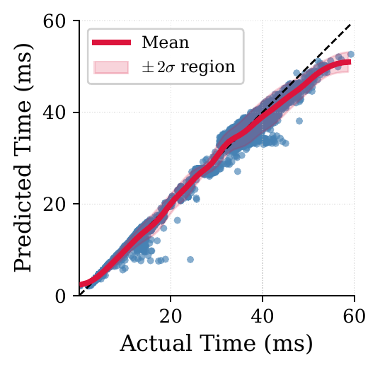
Two batches containing the same number of tokens can nevertheless have substantially different processing times. Increasing the decode context raises the decode-attention cost even when the number of newly processed tokens is unchanged, because each decode step must read a larger KV cache. Increasing the prior context similarly raises the cost of prefill attention, in addition to the quadratic self-attention within the prefill chunk itself. Consequently, batch processing time cannot be characterized by a single tokens-per-second rate: throughput depends on the composition of the batch and the context associated with its tokens.

Predicted versus measured token-batch processing time on Qwen3-0.6B across the range of batch compositions encountered during serving. The estimator achieves ≈4% mean absolute percentage error. Because SFS accumulates these batch-time predictions to estimate TTFT, their accuracy directly determines the fidelity of the resulting latency estimate.

Incorporating latency into the routing objective

With latency estimates available, the routing objective can account for response quality, monetary cost, and latency jointly. The accuracy–cost component follows the standard utility formulation: for query $q_i$ at instance $j$,

\[\widehat{U}_{i,j}(\lambda) \;=\; \widehat{\textrm{acc}}_{i,j} \;-\; \lambda\, \widehat{\textrm{cost}}_{i,j}\]

where $\lambda \ge 0$ controls the tradeoff between response quality and monetary cost. Accuracy is predicted using a LightGBM regressor over inexpensive prompt-derived features: hashed token vectors projected to 16 dimensions with PCA, together with token counts, sentence counts, and task-type indicators. The regressor is trained on LLM-as-a-judge scores. The same feature set is used for output-length prediction, which in turn supports both cost estimation and the decode-length inputs required by SFS.

Latency is imposed as a constraint. Each query has a TTFT target $\tau_i$; the feasible set contains instances predicted to satisfy this target, and the router selects the highest-utility feasible instance. If no instance is feasible, it falls back to the instance with the smallest predicted latency:

\[m(i) \;\leftarrow\; \operatorname*{arg\,max}_{j\in\mathcal{J}:\; \widehat L^{\textrm{ttft}}_{i,j}(t)\,\le\, \tau_i} \widehat U_{i,j}(\lambda)\]

Evaluation requires a metric that accounts for whether utility is delivered within the latency target. We therefore use OnTimeUtility, defined as mean realised utility with latency violations assigned zero utility:

\[\textrm{OnTimeUtility}(\lambda) = \frac{1}{N}\sum_{i=1}^{N} U_{i,m(i)}(\lambda)\, \mathbf{1}\!\left\{L^{\textrm{ttft}}_{i,m(i)} \le \tau_i\right\}\]

A Lagrangian relaxation replaces the hard latency constraint with a penalty $\delta$ on predicted latency, $\operatorname*{arg\,max}_j \big(\widehat U_{i,j}(\lambda) - \delta\,\widehat L^{\text{ttft}}_{i,j}(t)\big)$. Sweeping $\delta$ traces the utility–latency frontier. Setting $\delta = 0$ exactly recovers latency-agnostic routing, so that baseline appears naturally as one operating point on the same objective.

Experimental setup

We evaluate three Qwen3 models spanning a broad capability range: Qwen3-0.6B and Qwen3-8B are each deployed on one H100, while Qwen3-32B is deployed on two H100s using tensor parallelism. All experiments use vLLM; adapting SFS to another serving framework requires replacing the corresponding batching and scheduling logic. Generated responses are evaluated with LLM-as-a-judge using Gemini 3.1 Pro Preview.

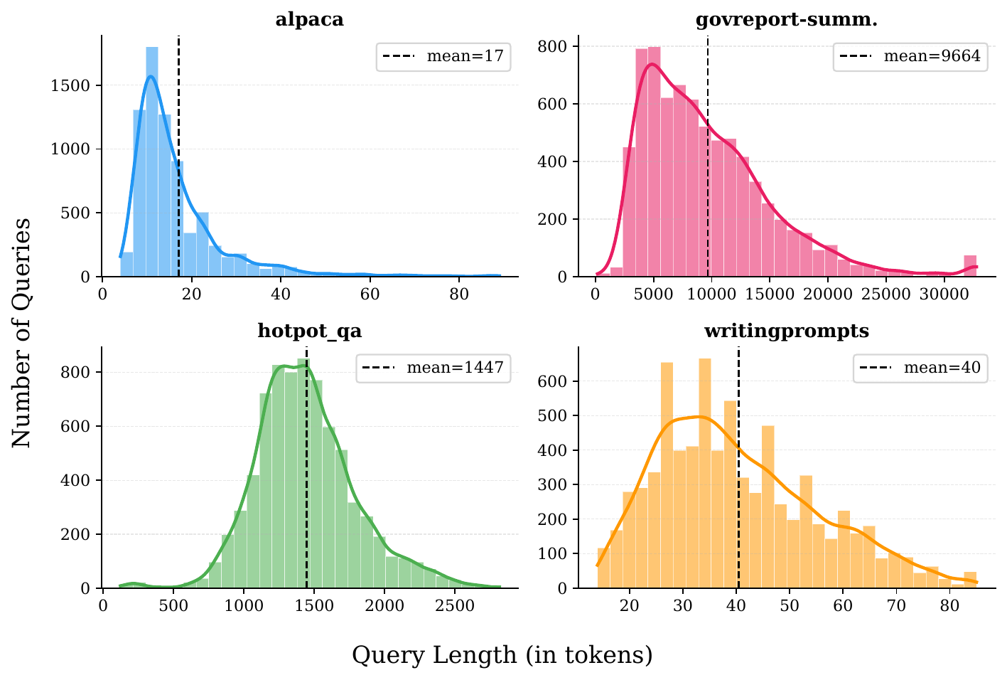
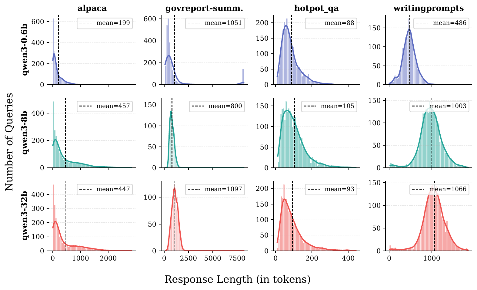
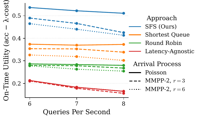
Queries are sampled from four tasks selected to span the prompt-length and response-length space: Alpaca (short prompt, short response), HotpotQA (long prompt, short response), GovReport-Summarization (long prompt, long response), and WritingPrompts (short prompt, long response). Prompt lengths range from roughly $10$ to $10^4$ tokens and response lengths from $10^2$ to $10^3$ tokens, producing a heterogeneous serving workload. The main experiments use Poisson arrivals, with a Markov-modulated Poisson process used to evaluate robustness to bursty traffic.

Workload length distributions. Prompt lengths (left) vary by roughly three orders of magnitude across tasks, while response lengths (right) depend on both the task and the model. This heterogeneity is important for latency estimation: a single tokens-per-second statistic cannot accurately characterise an instance processing a short Alpaca prompt and a multi-thousand-token GovReport prompt within the same serving workload.

Per-task response-quality scores (LLM-as-a-judge, %) and per-token prices. These values create meaningful routing tradeoffs across the model pool: the quality gap between Qwen3-0.6B and Qwen3-32B is substantially larger on WritingPrompts than on Alpaca, while Qwen3-32B costs roughly 3.7× more per output token than Qwen3-8B. Thus, no single model dominates across both response quality and monetary cost.

Task	Qwen3-0.6B	Qwen3-8B	Qwen3-32B
Alpaca	53.49	82.67	88.85
GovReport-Summarization	29.02	86.62	95.93
HotpotQA (distractor)	40.98	88.28	92.69
WritingPrompts	17.73	57.47	80.69
Aggregate	35.31	78.76	89.54
Prompt price, USD per M tokens	0.044	0.072	0.287
Response price, USD per M tokens	0.173	0.287	0.640

TTFT targets are generated as a linear function of prompt length with small random variation, $\tau_i \approx 158 + 3.5\times10^{-3} p_i$ ms, clipped to $[150, 1120]$ ms. The resulting targets are stringent enough to expose congestion-induced violations while remaining achievable for lightly loaded instances.

The baselines represent the two conventional sides of the problem. Round Robin and Shortest Queue provide load balancing without modelling response quality or cost, whereas Latency-Agnostic routing maximises utility without observing instance workloads.

Results

Performance under increasing offered load

Left: OnTimeUtility as the offered load increases. SFS achieves the highest OnTimeUtility at every evaluated arrival rate, with a 33% improvement in area under the curve over the best baseline and a 46% improvement at 5 q/s. Latency-Agnostic routing is competitive at low load but degrades as its preferred model instances saturate; Shortest Queue maintains low latency but cannot exploit query-specific model utility. Right: SFS maintains higher latency-constraint attainment as load increases, allowing a larger fraction of predicted utility to be realised on time.

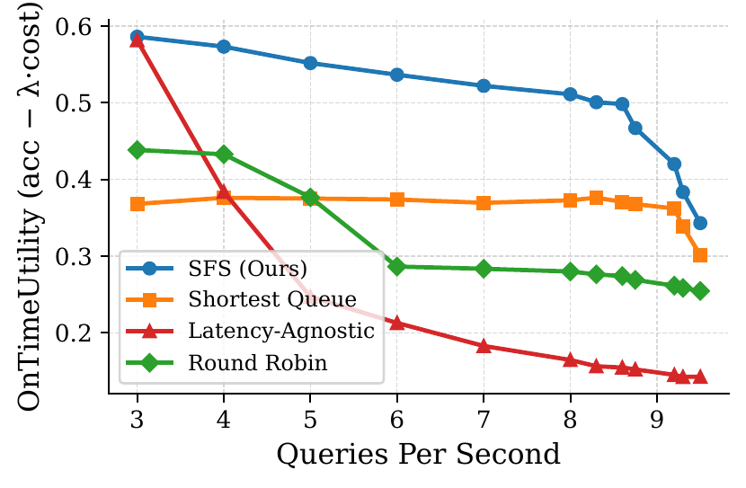
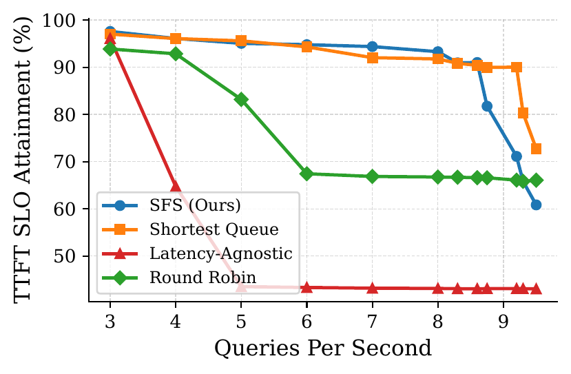
The behaviour of Latency-Agnostic routing illustrates why latency must be included in the model-selection decision. At low load, when congestion is negligible, selecting the highest-utility instance is appropriate. As load increases, however, the same policy concentrates requests on preferred instances and loses its utility advantage through latency violations.

Controlling the utility–latency tradeoff

Sweeping the latency penalty $\delta$ produces a controllable utility–latency frontier at 8 q/s. The horizontal axis is logarithmic and spans three orders of magnitude. The latency-agnostic router, corresponding to $\delta = 0$, attains its highest utility at an average TTFT of over 200 seconds. At the low-latency end, SFS achieves 40% higher utility than Shortest Queue at comparable TTFT, while Round Robin lies below the SFS frontier in both utility and latency.

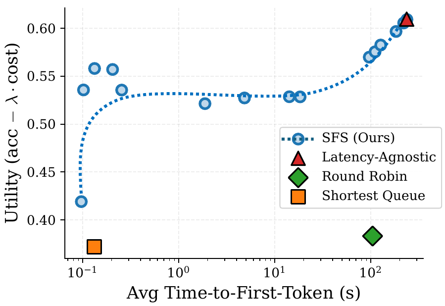
This result highlights an important advantage of the joint objective. The baseline policies correspond to fixed operating points, whereas latency-aware routing exposes a continuum of utility–latency tradeoffs controlled by $\delta$.

Routing composition by task

Fraction of queries assigned to each model instance by task at 8 q/s. Shortest Queue and Round Robin produce nearly identical routing compositions across tasks, reflecting their lack of query-specific model preferences. Latency-Agnostic routing is task-dependent but highly concentrated: it sends almost no requests to Qwen3-0.6B and assigns entire tasks predominantly to a single model. SFS remains task-dependent while adapting to congestion, routing approximately 37% of long-prompt GovReport requests to the smaller model when larger instances are congested, while continuing to favour Qwen3-32B for WritingPrompts, where its response-quality advantage is largest.

Bursty arrivals and estimator overhead

Left: Robustness to correlated arrivals using a two-state Markov-modulated Poisson process with high-to-low arrival-rate ratios $r = 3$ and $6$. The relative ordering of routing policies remains unchanged. Right: Wall-clock overhead of SFS, which lies on the routing critical path. Mean simulation time is approximately $10^{-4}$ s, three to four orders of magnitude smaller than the TTFTs being predicted.

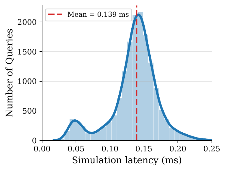
Low estimator overhead also depends on the system implementation. After each token iteration, every model instance publishes a compact workload snapshot to shared memory. Snapshots are marked in-progress or complete so that the router reads only consistent state without stalling the serving engine. The router retains the latest complete snapshot from each instance and simulates forward from that state. The batching simulation is approximately 300 lines of C++ within a ~3.6K-line Python/C++ implementation; porting SFS to another serving framework primarily requires adapting this scheduling simulation.

Average-case estimation without workload visibility

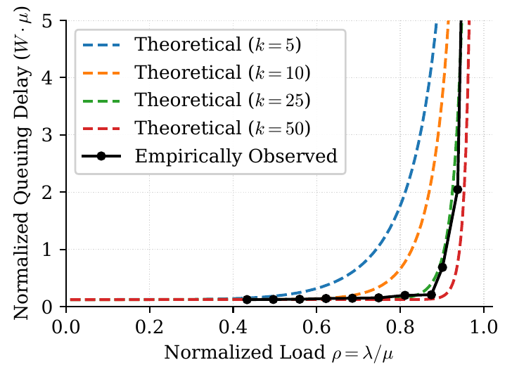
SFS assumes access to real-time workload snapshots. This information may be unavailable when, for example, a router sends requests to third-party cloud endpoints. In this setting, the paper develops an average-case approximation based on a Limited Processor Sharing (LPS) queue. Up to $k$ queries are served concurrently and share compute capacity, while additional requests wait in FCFS order. This abstraction better reflects autoregressive serving than a single-server queue because concurrency is explicit but bounded, and per-request token generation slows as more sequences share the GPU. With arrival rate $\alpha_j$, service capacity $\mu_j$, and utilisation $\rho_j = \alpha_j/\mu_j < 1$, the expected waiting time is

\[\widehat W^{\textrm{avg}}_{i,j} = \frac{(\alpha_j/\mu_j)^k}{\mu_j-\alpha_j}\]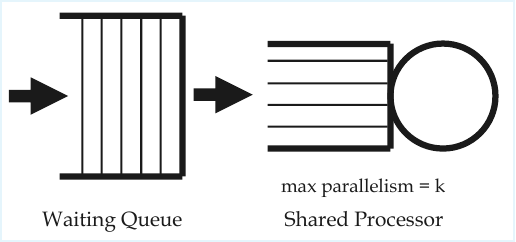

The Limited Processor Sharing abstraction (left) and its empirical fit (right). Measured TTFT on Qwen3-0.6B follows the qualitative growth of LPS waiting time as load increases; the observed time-average parallelism in this deployment is k ≈ 25. The approximation is necessarily coarser than SFS because it uses time-averaged rates rather than the instantaneous workload state, but it requires no visibility into the serving framework.

Scope and limitations

The central claim is deliberately focused: latency should be incorporated into the routing objective rather than delegated entirely to a lower systems layer, and the required latency estimates can be obtained efficiently by simulating the serving framework instead of compressing its state into a single throughput statistic. In our experiments, joint accuracy–cost–latency routing achieves over 40% higher utility than standard load balancing at comparable latency.

Several directions remain open. First, our primary objective optimises TTFT, which is appropriate for interactive responsiveness but does not fully characterise workloads whose quality of service depends on completion time. End-to-end latency is more sensitive to decode-length prediction error because the full generation horizon must be modelled. Second, model placement is fixed in our evaluation; jointly optimising routing decisions and model placement across heterogeneous hardware is a natural extension. Finally, SFS assumes that the workload state of each candidate instance can be represented consistently. With multiple independent routers sharing the same instance pool, each router perturbs the state being simulated by the others, creating an additional coordination problem that is not modelled in the current system.

The simulation on this page is a re-implementation for exposition. It uses the same batching policy and batch-time model as the paper, but illustrative coefficients and an intentionally equalised instance pool. Its purpose is to isolate and visualise the routing-induced failure mode rather than reproduce the measured experimental results above. The released system is available at github.com/akaashrp/sfs.

Cite this work

@article{patel2026beyond,
  title   = {Beyond Accuracy and Cost: Latency-Aware {LLM} Query Routing
             for Dynamic Workloads},
  author  = {Patel, Shivam and Parthasarathy, Akaash R. and
             Mallick, Ankur and Joshi, Gauri},
  journal = {arXiv preprint arXiv:2607.18253},
  year    = {2026},
  url     = {https://arxiv.org/abs/2607.18253}
}

← All publications