Publications LOCUS
LOCUS: Low-Dimensional Model Embeddings for Efficient Model Exploration, Comparison, and Selection
1Carnegie Mellon University† Corresponding author
A rapidly expanding model ecosystem
More than 300,000 text-to-text models are published on HuggingFace, and the ecosystem continues to expand. These models differ substantially in size, architecture, training data, and specialization. This heterogeneity is precisely what makes the model pool valuable — a 7B math model can outperform a 70B generalist on arithmetic at a tenth of the cost — but it also makes systematic model management increasingly difficult. Practical questions arise immediately: Which models are near-duplicates? Which small subset should be deployed? If a preferred model is unavailable, what is the closest substitute? When a new model is introduced, where does it belong relative to the existing pool?
These are fundamentally problems of model comparison, and a single leaderboard score is insufficient to address them. What is needed is a representation in which heterogeneous models can be placed in a common space, compared quantitatively, and searched efficiently. LOCUS adopts a simple representation for this purpose: each model is assigned a single fixed-dimensional vector.
\[m \;\longmapsto\; z_m \in \mathbb{R}^{d}\]The remaining question is how this vector should be constructed. Model parameters are an obvious source of information, but they are difficult to compare across heterogeneous architectures and are unavailable for proprietary API models. Output logits similarly depend on model-specific tokenization. In contrast, behavioural evaluations provide a model-agnostic interface: submit a query and assign a score to the resulting response. LOCUS therefore constructs model embeddings from evaluations alone. For a model $m$ evaluated on a set of queries $\mathcal{Q}_m$, where each query $x$ has a sentence encoding $\phi(x)\in\mathbb{R}^{d_\phi}$ and an evaluation score $y^{(m)}(x)\in[0,1]$ (typically binary correctness), the input is the set
\[S_m \;=\; \big\{\,(\phi(x_i),\; y^{(m)}(x_i))\,\big\}_{x_i \in \mathcal{Q}_m}\]and the output is a single model embedding. The remainder of the method follows from the construction of this mapping.
Desiderata for model embeddings
The use cases above impose several requirements that are individually natural but challenging to satisfy simultaneously:
- Black-box compatible — require only queries and evaluation scores, without access to weights, activations, or logits.
- Compatible with varying evaluations — models need not be evaluated on a common query set.
- Sample efficient — produce informative representations from few evaluations and improve as additional evaluations become available.
- Training-free onboarding — adding a model must not require optimizing model-specific parameters or modifying previously computed embeddings.
- Predictive — embeddings should support accurate performance prediction on unseen queries.
- Geometrically meaningful — cosine or Euclidean proximity should reflect model similarity.
Prior approaches broadly fall into two categories, each satisfying a complementary subset of these desiderata. Parametric methods — EmbedLLM, IRT-Net, and JE-IRT — treat each model embedding as a free parameter optimized jointly with a correctness predictor. These methods can predict performance accurately, but the resulting embedding is not uniquely determined by the evaluation data because it is obtained through stochastic optimization. Nonparametric methods such as LLM-DNA instead compute embeddings using fixed geometric operations, yielding deterministic representations, but require all models to be evaluated on the same queries, cannot naturally refine an embedding as additional evaluations arrive, and do not provide an associated correctness predictor.
| Method | Training-free embeddings | Correctness prediction | Varying eval queries |
|---|---|---|---|
| EmbedLLM | ✗ | ✓ | ✓ |
| IRT-Net | ✗ | ✓ | ✓ |
| LLM-DNA | ✓ | ✗ | ✗ |
| LOCUS | ✓ | ✓ | ✓ |
Instability of fitted per-model embeddings
Training-free onboarding is particularly important for preserving a consistent embedding geometry. Consider an EmbedLLM-style setting in which the correctness predictor $G_\psi$ is frozen and the embedding of a newly introduced model is optimized by gradient descent. If this optimization is repeated using evaluation data identical to that of an already embedded model, the regenerated embedding would ideally reproduce the original representation. In practice, it does not.
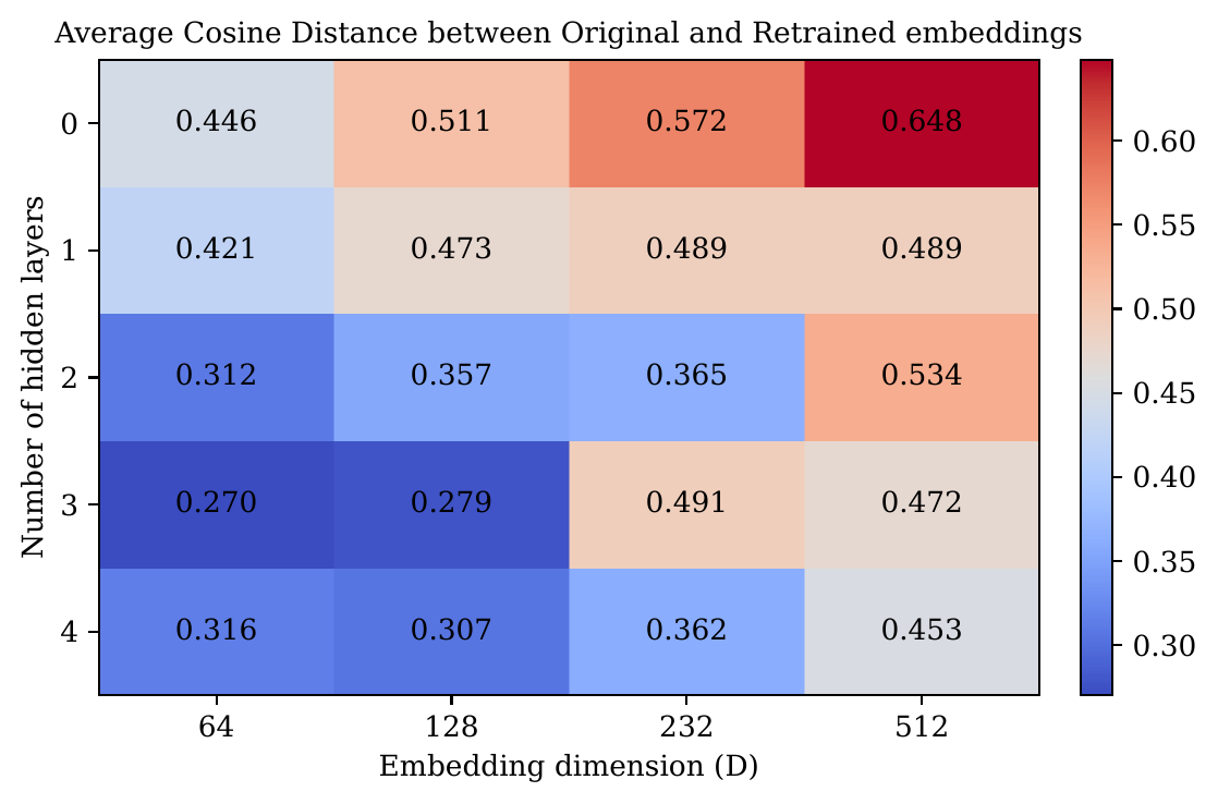
This non-uniqueness undermines distance-based analyses. Nearest-neighbour retrieval, clustering, and similarity search implicitly assume that identical model behaviour maps to the same representation. LOCUS enforces this property by construction: the embedding is the output of a fixed function of the evaluation set, so identical evaluations produce identical embeddings deterministically.
LOCUS: an attention encoder over evaluations
The evaluation collection $S_m$ is naturally a set: it has no intrinsic ordering and its cardinality can vary across models. These properties motivate the architecture. LOCUS uses a set encoder $F_\theta$ to map $S_m$ to a fixed-dimensional vector, together with a lightweight correctness predictor $G_\psi$ that maps a model embedding and query encoding to a correctness probability.
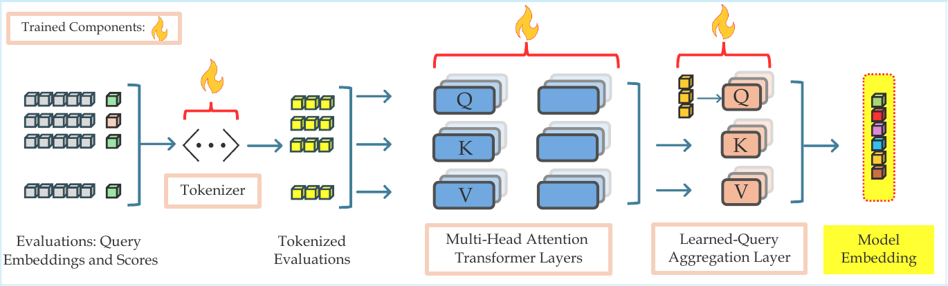
Step 1: tokenize each evaluation
A trained MLP $h_\omega$ maps each (query encoding, score) pair to a $d$-dimensional token, placing heterogeneous inputs in a shared representation space suitable for attention:
\[t_i^{(m)} \;=\; h_\omega\!\big(\phi(x_i),\; y^{(m)}(x_i)\big) \in \mathbb{R}^{1\times d}\]Stacking these tokens as rows gives $X_m^{(0)} \in \mathbb{R}^{n_m \times d}$, where $n_m = |S_m|$ denotes the number of evaluations available for model $m$. The subsequent architecture does not require $n_m$ to be shared across models.
Step 2: attention through a latent bottleneck
Direct self-attention over $n_m$ tokens has $\mathcal{O}(n_m^2)$ computational cost, which becomes restrictive when a model has thousands of evaluations. LOCUS instead introduces $r \ll n_m$ learned latent vectors $U^{(\ell)} \in \mathbb{R}^{r \times d}$. Each layer first compresses information from the evaluation tokens into the latents and then broadcasts the latent representation back to the evaluation tokens:
\[H_m^{(\ell)} = \mathrm{TBlock}\big(U^{(\ell)},\, X_m^{(\ell-1)},\, X_m^{(\ell-1)}\big) \in \mathbb{R}^{r\times d}\] \[X_m^{(\ell)} = \mathrm{TBlock}\big(X_m^{(\ell-1)},\, H_m^{(\ell)},\, H_m^{(\ell)}\big) \in \mathbb{R}^{n_m\times d}\]This reduces the attention cost to $\mathcal{O}(n_m r)$ — linear in the number of evaluations for fixed $r$ — while retaining global information flow through the latent bottleneck.
Step 3: aggregate with a learned query
A single learned query vector $s \in \mathbb{R}^{1\times d}$ attends over the final token representations and produces the model embedding:
\[z_m \;=\; \mathrm{TBlock}\big(s,\; X_m^{(L)},\; X_m^{(L)}\big) \in \mathbb{R}^{1\times d}\]Because the architecture uses no positional encodings and performs aggregation through attention rather than position-dependent indexing, $z_m$ is permutation invariant: reordering the evaluations does not change the embedding. This invariance is an exact architectural property rather than one learned approximately during training; the demonstration below verifies it numerically on the released checkpoint.
Step 4: predict correctness
To support downstream model selection, the embedding must be translated into query-specific performance estimates. A two-layer MLP $G_\psi$ takes a model embedding and query encoding as input and returns a correctness probability:
\[\widehat{p}_\psi\big(y^{(m)}(x)\!=\!1 \,\big|\, z_m, \phi(x)\big) \;=\; \sigma\big(G_\psi(z_m, \phi(x))\big)\]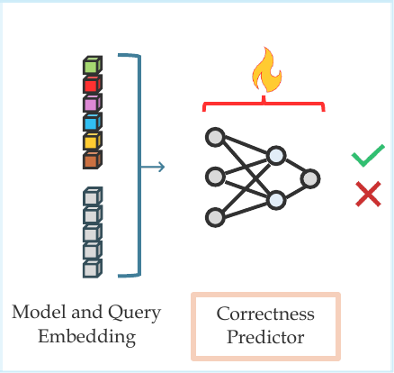
The encoder and predictor are trained jointly by minimizing binary cross-entropy. Each optimization step samples a mini-batch of models; for each model, an encoder subset $S_m^{\mathrm{enc}}$ is used to construct the embedding, while an independently sampled decoder batch $S_m^{\mathrm{dec}}$ provides the prediction targets:
\[\min_{\omega,\theta,\psi}\; \mathbb{E}_{m}\, \mathbb{E}_{x \sim S_m}\; \mathrm{BCE}\big(\widehat{p}^{(m)}(x),\, y^{(m)}(x)\big)\]Training on subsets of varying cardinality exposes the encoder to different values of $n_m$, enabling inference with variable-sized evaluation sets.
Onboarding a new model
- Evaluate $m_{\text{new}}$ on available queries and record their scores. ≈128 evaluations typically suffice
- $z_{m_\text{new}} \leftarrow F_\theta(S^{\text{enc}}_{m_\text{new}})$ a single forward pass
Not required
- Optimizing model-specific parameters. none are introduced
- Recomputing or modifying any existing $z_m$. existing embeddings remain unchanged
Interactive · one model, its evaluations, and the vector they produce
What this sample says the model can do n = 128
Fraction of that benchmark's questions the model answered correctly — green above 50%, red below, white at 50%. A dashed cell means the sample happened to contain no questions from that benchmark. The encoder never sees the benchmark names; they are shown only to make the estimate legible.
The embedding z ∈ ℝ128
- Distance to the 4,096-evaluation reference
- —
- Typical distance to a different model
- —
- Attention cost, r = 64 bottleneck vs plain
- —
Convergence to the reference embedding
Experimental setup
All experiments use the evaluation matrix released with EmbedLLM, comprising 112 language
models spanning base, chat, and finetuned specialists from approximately 1B to 72B
parameters. The models are evaluated on queries drawn from 10 public benchmarks —
MathQA, LogiQA, MedMCQA, PIQA, TruthfulQA, MMLU, GSM8K, GPQA, ASDiv, and SocialIQA.
Queries are encoded with all-mpnet-base-v2 into $\mathbb{R}^{768}$; ablations with three
additional sentence encoders are reported in the appendix.
The encoder uses $L=2$ latent-bottleneck blocks with 4-head attention and $r=64$ latent vectors, followed by the aggregation block. The embedding dimension is $d=128$, and the correctness predictor is a two-layer MLP with hidden width 64. Baselines are EmbedLLM and IRT-Net, both of which learn per-model embeddings through backpropagation. Test queries are never used to construct model embeddings and are reserved exclusively for evaluation.
Two metrics are used throughout. Correctness prediction accuracy thresholds $\widehat{p}^{(m)}(x)$ at $0.5$ and measures agreement with observed labels across model–query pairs. Routing accuracy assigns each query to the model with the highest predicted correctness probability and measures the fraction of routed queries for which the selected model is correct.
Results
Routing and correctness prediction
| Approach | Routing accuracy (%) | Corr. prediction (%) | ||||
|---|---|---|---|---|---|---|
| 256 | 512 | 1024 | 256 | 512 | 1024 | |
| LOCUS | 61.90 | 62.97 | 64.70 | 68.31 | 68.33 | 70.03 |
| EmbedLLM | 58.80 | 59.47 | 59.60 | 67.33 | 68.12 | 69.47 |
| IRT-Net | 59.57 | 60.17 | 63.37 | 67.38 | 69.07 | 70.12 |
Sample efficiency
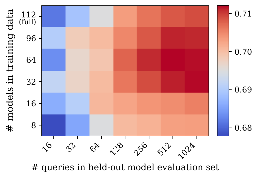
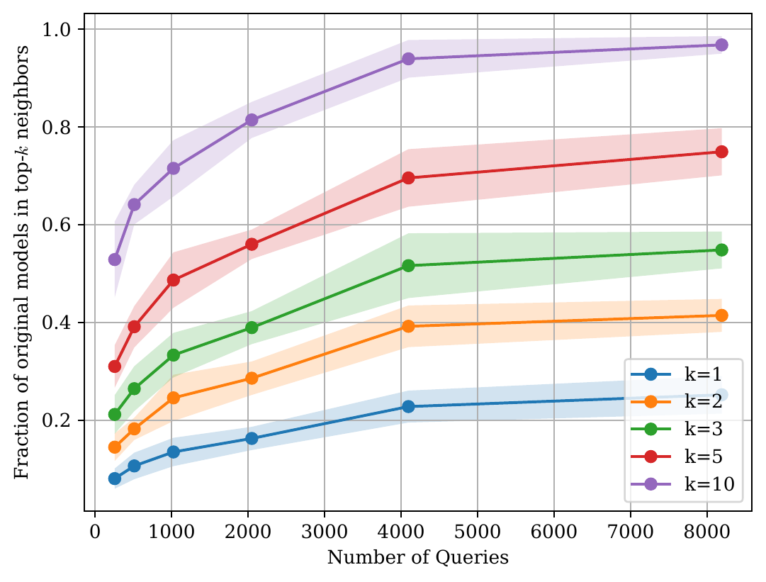
The advantage becomes larger in the low-evaluation regime, which is operationally important because each additional evaluation incurs an inference call to a model in the pool.
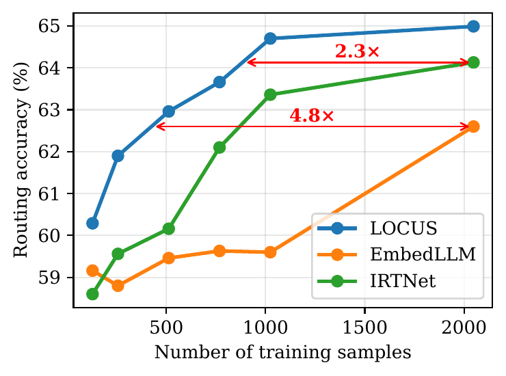
A similar trend appears during test-time onboarding, where the relevant quantity is the number of evaluations required to obtain an informative embedding for a new model.
Robustness to evaluation-set composition
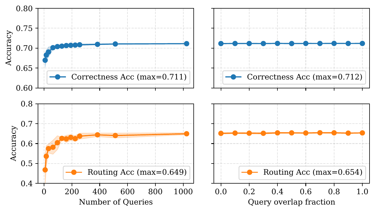
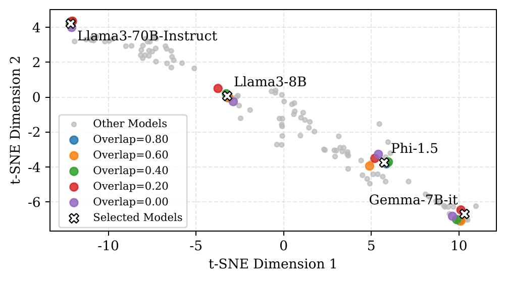
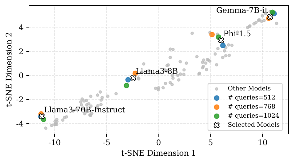
Different models are rarely evaluated on identical query sets, so useful model embeddings should remain stable when the available evaluations are resampled. We examine two forms of variation: changing which queries are used at a fixed evaluation count, quantified by the overlap fraction $\alpha$ with a reference set, and changing how many evaluations are available.
Embedding distance reflects behavioural similarity
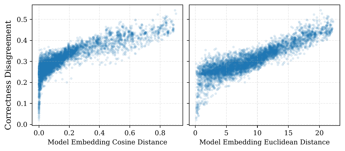
The downstream utility of the embedding space depends on whether geometric distance tracks behavioural differences between models. We evaluate this directly by computing, for each model pair, both the embedding distance and the correctness disagreement rate — the fraction of test queries on which their binary correctness labels differ.
| Correlation | Cosine distance | Euclidean distance |
|---|---|---|
| Pearson $\rho$ | 0.845 | 0.887 |
| Spearman $r_s$ | 0.886 | 0.876 |
| Kendall $\tau$ | 0.714 | 0.702 |
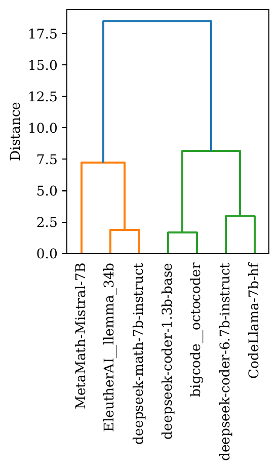
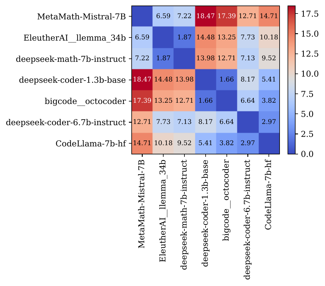
The geometry also reveals structure that is not provided as supervision. Hierarchical clustering based on pairwise embedding distances separates math-finetuned and code-finetuned model families without access to these family labels.
Inspecting the embedding space
The interactive visualization below provides a direct view of the learned geometry. It contains all 112 model embeddings from the released checkpoint, together with their nearest neighbours, per-benchmark accuracy profiles, and correctness agreement statistics. The three-dimensional projection can be rotated and zoomed, which helps disambiguate points that overlap in any single two-dimensional view. The two interaction modes correspond to the downstream applications discussed next.
Interactive · all 112 model embeddings, in three dimensions
Loading…
Drag to rotate · + / − to zoom · click a model to see its neighbours
Selected model
—
Accuracy by benchmark
Nearest neighbours — click a row to follow
Routing accuracy of the selected portfolio
Models chosen
Applications of the embedding geometry
Nearest neighbours as model substitutes
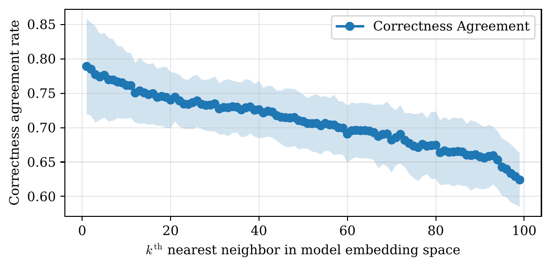
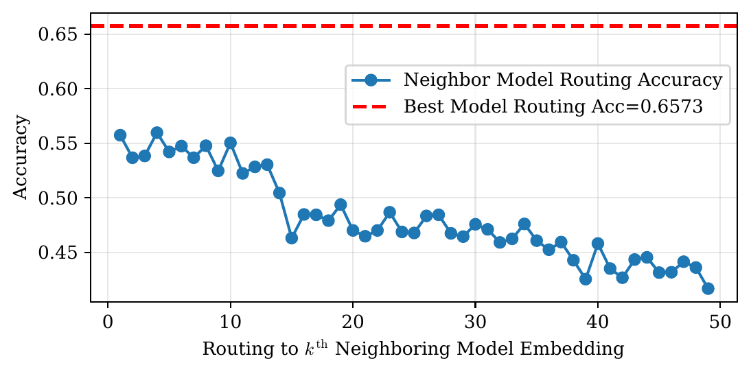
A routing system may select a model that subsequently becomes overloaded, unavailable, or ineligible under a deployment policy. In the absence of query-specific scores for all alternatives, a geometrically meaningful model space provides a principled basis for selecting a substitute. Ranking each model’s neighbours by embedding distance and measuring correctness agreement on common queries evaluates whether this substitution preserves behaviour.
Model portfolio selection
Deploying all 112 models is often impractical. A more relevant systems question is which small subset should be retained while preserving the capabilities of the full pool. The embedding space enables this selection without evaluating every candidate subset: choose models that cover the space, using geometric coverage as a proxy for coverage of distinct model behaviours.
Two classical facility-location objectives apply directly. k-center minimizes the maximum
distance from any model to the selected set, while k-medoids minimizes the average
distance. Under a total parameter budget rather than a model-count constraint, a
coverage-greedy rule selects the model with the largest marginal coverage gain
per parameter, thereby accounting explicitly for model size.
k-center that match the routing accuracy of all 112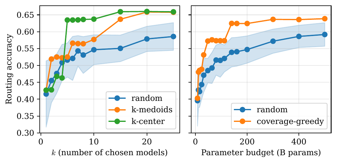
k-center saturates
at $k \approx 15$. Right: under a total-parameter budget,
coverage-greedy reaches near-full accuracy using a small fraction of the
pool's 1,930B parameters. Selection uses only $\{z_m\}$; no routing evaluation of
candidate subsets is required.Searching by a target capability profile
Because the encoder maps any evaluation set to a vector, it can also embed hypothetical evaluation profiles. Given a desired per-task accuracy profile, we can synthesize an evaluation set with matching task-wise rates, map it through $F_\theta$, and retrieve the nearest embeddings from the library of real models. This enables model search by a target capability profile rather than by model name or aggregate benchmark rank.
Identifying near-duplicate models
Deterministic embedding generation together with stability under resampling provides a natural fingerprinting signal. If two endpoints repeatedly map to nearly the same location across independently sampled evaluation sets, they may correspond to the same or closely related models. In the embeddings recomputed for this page, the nearest model pairs have cosine distances on the order of $10^{-5}$ or smaller and correspond to closely related model variants.
| Model pair | Cosine distance |
|---|---|
| ConvexAI/Luminex-34B-v0.2 · fblgit/UNA-SimpleSmaug-34b-v1beta | < 10−5 |
| rishiraj/CatPPT-base · bardsai/jaskier-7b-dpo-v5.6 | < 10−5 |
| berkeley-nest/Starling-LM-7B-alpha · openchat/openchat_3.5 | 2 × 10⁻⁵ |
| CultriX/NeuralTrix-bf16 · openchat/openchat_3.5 | 2 × 10⁻⁵ |
Computational cost
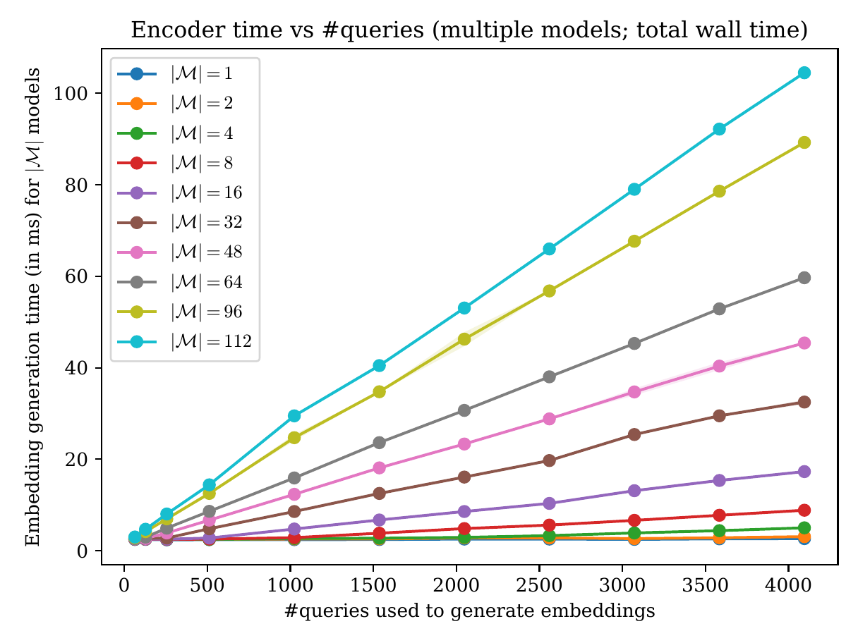
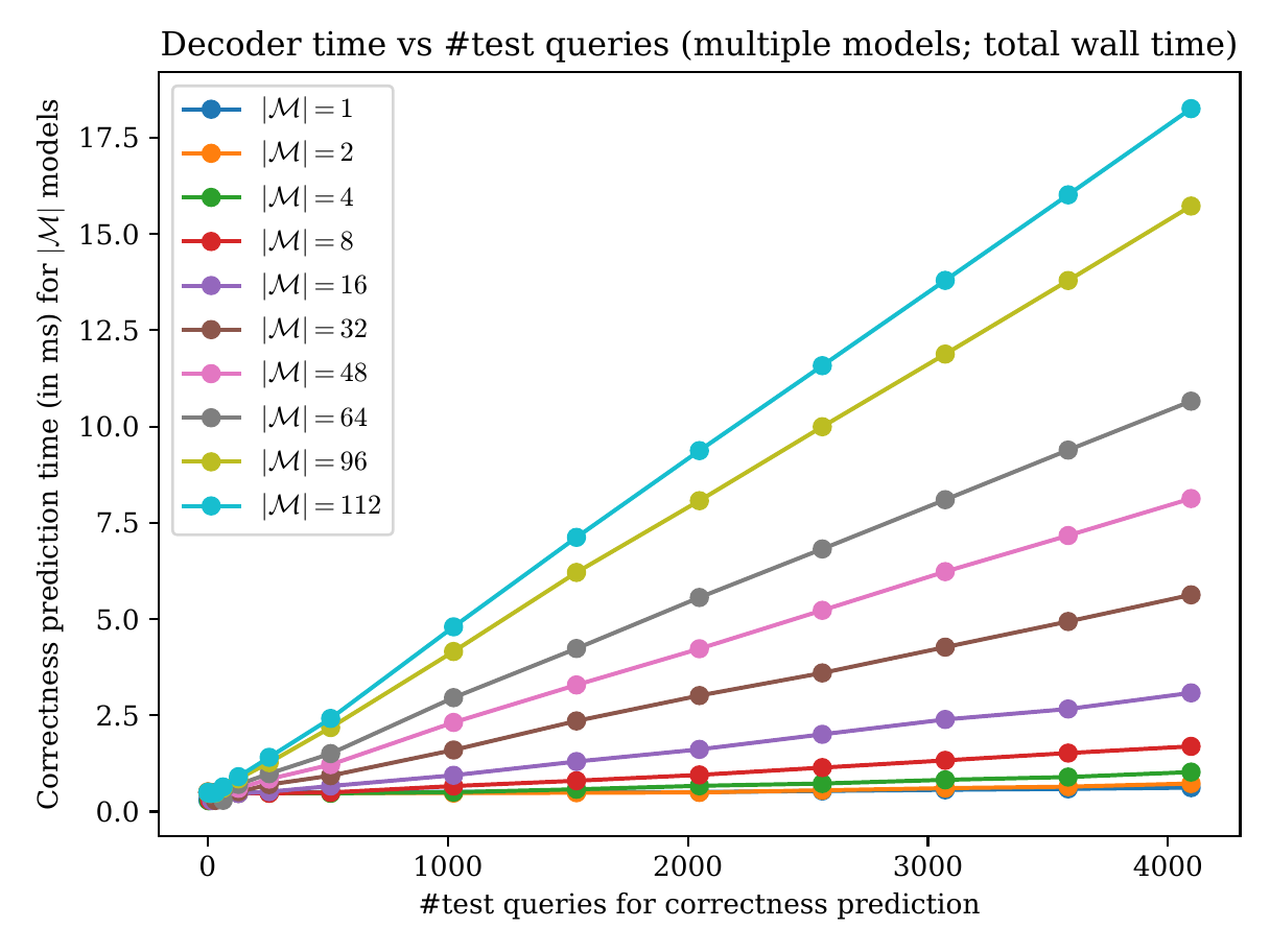
Empirical runtime measurements confirm the encoder’s linear scaling with evaluation-set size. Embedding the full 112-model pool from 4,096 evaluations per model takes approximately 100 ms on a single V100, while scoring 4,096 unseen queries against all 112 models takes approximately 20 ms. This overhead is two to three orders of magnitude below the seconds-scale latency of the corresponding language-model generations.
Summary
LOCUS represents a language model as a single low-dimensional vector computed from scored query evaluations by a trained attention encoder. Generating embeddings through a deterministic forward pass, rather than fitting model-specific parameters, provides several useful properties: new models can be onboarded without retraining or modifying existing embeddings, representations can be refined as additional evaluations accumulate, and identical evaluation sets map to identical vectors, making distance-based analyses reproducible.
Empirically, LOCUS is substantially more sample efficient than learned-parameter baselines (up to $4.8\times$ relative to EmbedLLM), requires roughly 128 evaluations to embed an unseen model, and produces a geometry that is strongly associated with behavioural similarity. Embedding proximity supports model fallback while retaining 85% of routing accuracy, hierarchical clustering recovers model families, and geometric coverage selects a 15-model portfolio that matches the routing accuracy of the full 112-model pool. Promising extensions include multimodal model representations and adaptive selection of which queries should be evaluated when onboarding a new model.
Cite this work
@inproceedings{
  patel2026locus,
  title     = {{LOCUS}: Low-Dimensional Model Embeddings for Efficient
               Model Exploration, Comparison, and Selection},
  author    = {Shivam Patel and William Cocke and Gauri Joshi},
  booktitle = {ICML 2026 Workshop on Adaptive Foundation Models},
  year      = {2026},
  url       = {https://arxiv.org/abs/2601.21082}
}